Nexus Motion Capture Software for Biomechanics and Gait Analysis
Data capture software designed for life sciences. With Nexus you can integrate inertial and markerless into your optical motion capture system.
Nexus 2.20 is available now!
Nexus is the most powerful all-inclusive modeling and processing tool for movement analysis on the market. Created specifically for the whole life sciences community, Nexus delivers precise, repeatable data and clinically validated model outputs.
We are leading the way in our field. Precisely synchronise inertial data with optical, add market-leading eye trackers or 3rd party video cameras into your system – how can you benefit from the latest capabilities of Nexus?
Easily calibrate and configure the system. Seamlessly connect mobile devices via the Vicon Control app. Prepare subjects by creating templates and calibrating pipelines, to allow data capture away from your desk. The data-processing engine automatically initializes the labeling of your subject, removing the need to label manually. Nexus can automatically detect gaps and display information about labeling quality, enabling quick data correction if needed.
Nexus enables you to capture movement, review trials, assess foot strikes and review data quality. Perform modeling, using PiG, CGM2 the Oxford Foot Model, or your own model. Input subject measurements for PiG or full body analysis. Incorporate external integrations such as EMG, force plates, and inertial sensors.
Save time with highly customizable, automated processing operations. You can review your processing history and quickly pull off reports. Create custom pipelines for common processing tasks. With direct native pipeline integration, you can process data using scripts created in Python, MATLAB and Vicon ProCalc.
Nexus can seamlessly integrate with Vicon’s market-leading IMU, Blue Trident. It’s wireless network device, Beacon, allows seamless synching across data types. By adding inertial sensors into the optical world, you can utilize and compare optical and inertial data in one platform.
Global angles are available on the Blue Trident sensor. Using OpenSense integration, joint angles can be calculated.
Open Sound Control is the protocol for communication among computer and sound synthesizers for networking technology. Nexus provides options for streaming data in OSC format, enabling live synchronized or offline. Data can be accessed by any platform that supports OSC for real-time control of sound and other media processing.
Tobii’s latest eye tracker is integrated into Nexus, enabling streaming of synchronized eye-gaze tracking with optical data.
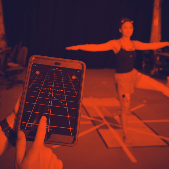
Gait Analysis & Rehabilitation
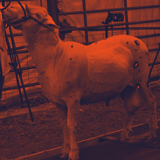
Animal Science
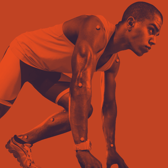
Sports Scientists
Biomechanists

| Current release version | Windows 11 | Windows 10 | Windows 7 | Linux | OSX |
| Shōgun 1.19 | 64 bit | 64 bit | x | x | x |
| Nexus 2.16 | 64 bit | 64 bit | x | x | x |
| Evoke 1.7.0 | 64 bit | 64 bit | x | x | x |
| Tracker 4.1.0 | 64 bit | 64 bit | x | x | x |
| Polygon 4.4.6 | 64 bit | 64 bit | x | x | x |
| Capture.U Desktop 1.3.1 | 64 bit | 64 bit | x | x | 10.12 |
| CaraLive 1.3.0 | 64 bit | 64 bit | 64 bit * | x | x |
| CaraPost 1.2.0 | 64 bit | 64 bit | 64 bit* | x | x |
| Pegasus 1.2.2 | 64 bit | 64 bit | 64 bit* | x | x |
| ProCalc 1.6.1 | 64 bit | 64 bit | x | x | x |
| ProEclipse 1.5.0 | 64 bit | 64 bit | x | x | x |
| DataStream SDK 1.12.0 | 64 bit | 64 bit | x | 64 bit | 10.11 |
| Bodybuilder 3.6.4 | 64 bit | 64 bit | x | x | x |
| Nexus Insight 1.0.0 | 64 bit | 64 bit | x | x | x |
Please do note:
1. Open the Network and Sharing Center and navigate to Change Adapter Settings. Vicon Vantage/Vero cameras are designated to one port. For each Vue (or Bonita Video) camera connected, there will be additional network port used.
2. Right click on the proper port and go into the Properties. The Local Area Connection Properties window will open. Make sure only Internet Protocol Version 4 (TCP/IPv4) is selected.
3. Select Internet Protocol Version 4 (TCP/IPv4) from the list and select Properties to assign the proper IP address.
a .Vantage/Vero cameras will have the following IP Address: 192.168.10.1 and Subnet Mask of: 255.255.255.0
b. The first VUE camera will have the following IP Address: 192.168.10.2 and Subnet Mask of 255.255.255.0
c. Any additional VUE cameras the last IP value is incrementally increased by one. For example, the second VUE camera will be 192.168.10.3.
Select OK to close out of the Internet Protocol Version 4 (TCP/IPv4) Properties. And OK again to close out of the Local Area Connection Properties. This will make sure all changes have been saved.
4. Feel free to rename the network port so it is easily identifiable. Such as ViconMX, VUE1 or VUE2
For further assistance please refer to the Configuring Ports section of the PCSetupforViconSystems.pdf found in Downloads > Documentation
Nexus documentation
Visit the Nexus documentation pages, for information including:
Nexus_2.20
File Name: Nexus_2.20.0+168415h_x64
With a host of automated features, intelligent processing, and flexible controls, Nexus 2 lets you focus on your research and not on your software.
Nexus 2.20 is a point release which focuses primarily on performance improvements for captures with FLIR cameras. Several important issues were also resolved to help improve the overall stability and reliability of the software.
New features and changes include:
* Support MATLAB version updated to 2025b
* Connection port for the NexusSDK can be specified using a command line option
* Integration of ProEclipse is now done using the NexusSDK and no longer requires an additional installer or registration of an ActiveX component
* A command line option can be be used to open Nexus with its default layout
* New control to suppress FLIR warnings about sharing an interface or USB controller
* CGM2 operations updated to call .py scripts rather than .exe
* Batch processing and Transcoding panels moved to more accessible locations
* Subject calibrator algorithm enhancements to help improve labeling
Addressed Issues:
* Nexus freezing and lagging after multiple captures with Video Payload set to JPEG (GPU)
* Fixed some issues with misreporting of capture availability when sources are disabled or have warnings
* Update to video buffer allocation to allow more of the capture buffer to be used
* Flir AOI (Applied) parameters remain fixed when adjusting the AOI commands
* Changing video payload setting between Uncompressed and JPEG(GPU) does apply to the first capture after the change
* Having the Communications panel undocked on opening and subsequently docking and undocking in some cases caused Nexus to crash.
* Live graph display only displays 100 frames of data.
* Potential fix for crash when graphing Combined force plates
* Key frame identification issue in AVI transcoding
* MATLAB script error in CreateViconGaitModelOutputs
* Default values of sound files not displaying properly in the Sounds dialog
* Oxford Foot Model marker diameter not being used by the pipeline operation
Requirements:
* Licensing: Nexus 2 license
* Operating system: Windows 11
Nexus_2.19
File Name: Nexus_2.19.0+166544h_x64
With a host of automated features, intelligent processing, and flexible controls, Nexus 2 lets you focus on your research and not on your software.
Nexus 2.19 is a point release which adds support for up to 12 video cameras as well as on-the-fly GPU compression and shared GPOs for video capture setups.
New features and changes include:
* 8+ Video Camera support (requires appropriate GPU and PC)
* GPO sharing amongst other FLIR cameras
* Additional Flir set issues
* Nexus buffer size parameter defaults have been updated; Buffer Size and Buffer Reserve defaults are now 4096 and 0.3 respectively
* Security updates (use https instead of http)
Addressed Issues:
* IMU World alignment orientation properties are not filling
* Save changes popup on entering Video Calibration mode leaves dirty flag on the System file
* Disabling a device output on a digital device with multiple outputs can lead to erroneous data on the other outputs
* Graph mean/stdev display can use the wrong range in device data in some cases if there is a frame offset in the data sources
* AGW Model templates are now installed to the expected folder so they appear in the appropriate place within the application
* Capture start on labeling or capture before start is now more reliable when subsampled video is being captured
* Transcoding using a pipeline operation can cause Nexus to deadlock when it is run with a Live system connected
Requirements:
* Licensing: Nexus 2 license
* Operating system: Windows 11
Nexus_2.18
File Name: Nexus_2.18.0+164370h_x64
With a host of automated features, intelligent processing, and flexible controls, Nexus 2 lets you focus on your research and not on your software.
Nexus 2.18 is a point release for Vicon Nexus which adds support for Valkyrie 6 (VK6) cameras and improves the performance of the FLIR cameras.
New features and changes include:
* Active Wand 4 support
* Video-only calibration
* Updated UI/UX for camera calibration workflow
* Changing the wand selection dropdown to a standard parameter
* Renaming of parameters for continuity with other applications
* Removal of deprecated parameters
* Removal of deprecated pipelines related to offline camera calibration
Addressed Issues:
* Export MOT fixes to export free vertical moment as an action rather than a reaction and to allow extended ASCII characters in the output file path
* Fixed an issue where the Flir area of interest was not staying central in all cases
* Fixed space bar hotkey
* Reset the custom model template folder to C:\Users\Public\Documents\Vicon\Nexus2.x\ModelTemplates, this folder had been erroneously set to C:\Users\Public\Documents\Vicon\Nexus2.x\Configurations\ModelTemplates in Nexus 2.17.
* Fixed batch processing issue where proEclipse nodes were not being accessed properly.
* 3rd Party License dialog is now displaying the license text rather than a blank window.
* Firmware update manager now launches when user elects to update firmware from the Check for * Firmware Updates dialog.
Requirements
* Licensing: Nexus 2 license
* Operating system: Windows 11
Nexus_2.16
File Name: Nexus_2.16.0.150876h_x64
With a host of automated features, intelligent processing, and flexible controls, Nexus 2 lets you focus on your research and not on your software.
Nexus 2.16 is a point release for Vicon Nexus, which is a *64-bit only* application that supports all Vicon Valkyrie cameras. Before upgrading, please ensure your system remains compatible.
New features and changes include:
Addressed issues:
Requirements:
Nexus_2.15
File Name: Nexus_2.15.0.145908h_x64.zip
With a host of automated features, intelligent processing, and flexible controls, Nexus 2 lets you focus on your research and not on your software.
Nexus 2.15 is a point release for Vicon Nexus, which is a 64-bit only application that supports the new Vicon Valkyrie cameras. Before upgrading, please ensure your system remains compatible.
New features and changes include:
Addressed issues:
Requirements:
Nexus_2.14
File Name: Nexus_2.14.0.139696h_x64.zip
With a host of automated features, intelligent processing, and flexible controls, Nexus 2 lets you focus on your research and not on your software.
Nexus 2.14 is a point release for Vicon Nexus, which is a *64-bit only* application. CGM2 has been updated and now uses Python 3. Before upgrading, please ensure your system remains compatible.
New features and changes include:
Addressed issues:
Requirements:
Nexus 64-bit_OpenGL
Nexus 2.13 and 2.16 (64-bit) is tested and fully supported with NVIDIA graphics processors. This is the Vicon-recommended graphics processor for PCs that are to run your Vicon system and Nexus software.
OpenGL_64-bit
Using other graphics processors is not recommended and may affect the performance of the software.
The OpenGL workaround for non-NVIDIA graphics processors is only available for Nexus 2.13-2.15. For Nexus 2.16, this third-party library may cause Nexus to stop responding.
If you experience issues with the software and you have been informed by Vicon Support that this is due to the graphics processor, note these points:
If an NVIDIA processor is not available and Nexus stops responding, the following workaround may help. It involves installing an additional file to the Nexus program directory. To do this, you need read/write access to this location and may require the help of an administrator.
This workaround may mitigate issues that are due to the graphics processor which you may experience while you’re running Nexus, however, performance, such as redraw and general navigation, may be adversely affected. This third-party library workaround has been tested on a limited number of Intel graphics cards for Windows 10 and not a supported solution.
Nexus_2.13
File Name: Nexus_2.13.0.138379h_x64.zip
With a host of automated features, intelligent processing, and flexible controls, Nexus 2 lets you focus on your research and not on your software.
Nexus 2.13 is a point release for Vicon Nexus, which is a 64-bit only application. The update includes support for FLIR video cameras and the H.264 video codec. Before upgrading, please ensure your system remains compatible.
New features and changes include:
Addressed issues:
Requirements:
Before you install Nexus 2, note the following limitations on supported systems:
Nexus 2 (Windows 10 configuration fully supported and tested) supports the following reference video options:
For the recommended and latest PC specifications, please refer to https://vicon.com/support/faqs/?q=what-are-the-latest-pc-specifications or contact Vicon Support
Nexus 2.13 does not support the use of Basler video cameras. To use Basler video cameras with Nexus, use Nexus 2.12.1 or earlier.
Link aggregation is used to describe various methods for using multiple parallel network connections to increase throughput beyond the limit that one link (one connection) can achieve. Link aggregation is supported in Tracker 1.3+, Nexus 1.8.5+, Blade 2+.
When setting up Link Aggregation ensure that you have the correct Network cards (Intel i340-T4 or the Intel i350-T4 cards) installed on your capture PC. Once you have the correct Network card(s) follow these steps:
1. Make sure your three network ports have fixed IP addresses 192.168.10.1, 192.168.10.2 and 192.168.10.3. A maximum of nine NICs are allowed (192.168.10.1 – 192.168.10.9 inclusive).
2. Connect the 192.168.10.1 and 192.168.10.2 ports to one Giganet/Power over Ethernet switch (POE) and 192.168.10.3 to the other Giganet/POE. You will need an extra cable connecting your Giganets/POEs.
3. Run Tracker/Nexus/Blade, set your workspace to Camera and select all the cameras in the System pane (you will need to expand Vicon Cameras). Please do note that there might be slight differences between the three applications.
4. Turn the Giganet/POE connected to 192.168.10.3 off then select all the cameras that just went red in the System pane.
Select the Destination IP Address drop-down and select 192.168.10.3.
5. Select the remaining (green) cameras then scroll down their Properties, select the Destination IP Address drop-down and select 192.168.10.2.
6. Turn the Giganet/POE connected to 192.168.10.3 back on. Select all the cameras in the System pane.
Save your System configuration.
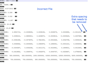
When you add a force plate in Nexus, you are also required to install the Calibration File into the appropriate dialogue box. The Calibration file generally comes with the device from the manufacturer. This can be a .Plt file or an .acl file for AMTI plates.
There may be occasion when the file located does not populate the drop down box on selection within Nexus.
In this instance, you may need to hand edit the file to remove any white space or extra characters, such as Commas and Carriage returns, in order for it to be read by Nexus.
Open the file in a text editor, and remove any white space and/or extra characters not required.

You can find the latest documentation for all current versions of software here:
Vicon Core Software will also install documentation/help guide when you install the software.
Once installed, launch the software and select Help > View Installed Help
The following software will install Help:
Nexus 2, Shōgun, Tracker 3, Blade 3, Pegasus, CaraLive, CaraPost, Polygon 4
There are four gap filling options available in Nexus 2.
Woltring (Quintic spline)
This has slightly different behaviour for the pipeline operation compared to the manual fill.
Both versions generate a quintic spline using valid frames around the gap as seed data. The gap is filled using the interpolated values from the spline. If there are insufficient frames surrounding the gap, the fill is rejected.
Pipeline
Searches backwards and forwards from the gap looking for (Number of Gap Frames / 2) + 5 consecutive valid frames on each side, but will accept a minimum of 5 valid frames on either or both sides if the preferred range is not available. Searches the entire length of the clip looking for the valid frame ranges.
Manual
Searches up to (Number of Gap Frames / 2) + 5 frames backwards and forwards from the gap. Requires a minimum of 10 valid frames in this range – these are not required to be consecutive.
Pattern
Manual fill operation only.
Generates linear interpolations between the valid frames either side of the gap and between the same frames in a donor trajectory. The interpolated value in the gap trajectory is then offset by the difference between the interpolated and true values in the donor trajectory. Mathematically:
Let F(t) be the value in the position of the trajectory to fill at frame t, and D(t) that of the donor trajectory. Let t0 and t1 be the valid frames before and after the gap, respectively. Then if we define the interpolated position V of trajectory Gat frame t as:
V(G(t)) = ( G(t1)-G(t0) ) * ( t – t0 ) / ( t1-t0 ) + G(t0)
then:
F(t) = V(F(t)) – V(D(t)) + D(t)
Rejects the fill if the donor trajectory has any invalid frames within the gap region, or if the donor or fill trajectory are invalid at either t0 or t1
Rigid Body
Takes a number of trajectories and assumes these move as a rigid body. The gaps in the selected trajectory are filled as if this trajectory is also a part of the same body. Manual filling is restricted to 3 donor trajectories and fills gaps in a single trajectory; the pipeline operation will use as many donor trajectories as possible, and will attempt to fill the gaps in each selected trajectory using all the other selected trajectories as donors.
Define the state at frame t as an (n x 3) matrix M(t) whose rows are the position vectors of the donor trajectories, P(t) as the position of the fill trajectory, and tx as a reference frame in which the positions of the donors and fill trajectory are all known.
We transform M into M by subtracting the mean value of the column i from each row entry M(t)(i,j):
M(i,j) = M(i,j) – O(j), where O(j) = ( (i=1->n) ∑ M(i,j) / n )
We then create a covariance matrix C = M(tx)’ M(t) and perform an SVD such that C = U S V*
We take L to be the the identity matrix, except that if det( V U* ) < 0, then L(3,3) = -1. Then we can generate a rotation matrix R(tx) = V L U* (This is effectively the Kabsch algorithm to find the optimal rotation between two point clouds)
The interpolated position at frame t based on reference frame tx is then defined as:
G(t, tx) = R(tx) ( P(t) – O(tx) ) + O(t)
and
F(t) = ( G(t, t1) – G(t, t0) ) * ( t – t0 ) / ( t1 – t0 ) + G(t, t0)
where t0 and t1 are the valid frames before and after the gap, respectively.
The fill is rejected if there are fewer than 3 valid donor trajectories at any frame t0 <= t <= t1, or if the trajectory to fill is invalid at t0 or t1.
Kinematic
Determines the fill based on the position and orientation of a segment. The manual operation operates on a single selected trajectory, while the pipeline operation attempts to fill gaps in all trajectories associated with the selected segment.
The mathematics of this operation are simply:
G(t, tx) = R(t) R(tx)’ ( P(t) – O(tx) ) + O(t)
and
F(t) = ( G(t, t1) – G(t, t0) ) * ( t – t0 ) / ( t1 – t0 ) + G(t, t0)
where R(t) is the rotation matrix defining the orientation of the segment in the world at frame t, O(t) is the origin position of the segment at frame t, and t0 and t1 are the valid frames before and after the gap, respectively.
The fill is rejected if there are no kinematics for the selected segment at any frame t0 <= t <= t1, or if the trajectory to fill is invalid at t0 or t1.
To configure force plates for analog data capture:
1. Go to the Resources pane > Systems tab, click the Go Live button.
2. In the System tab, right-click the Devices node, point to Add Analog Device and select the proper force plates.
The selected force plate node automatically expands to display the newly created device. If the appropriate type is not displayed, contact Vicon Support.
3. In the Properties section at the bottom of the System resources pane, select Show Advanced.
4. In the General section
5. In the Source section
Please Note: Expand force plate node to expose the Force, Moment and CoP (Center of Pressure) channels. A Green Arrow indicated a connected source device and a Yellow yield indicates that a channel has not been assigned a pin.
6. In the Dimensions section, add in values from force plate manufacturer’s manual if not already entered
7. In the Positions section, position the force plate in respect to the wand and the origin of the plate.
8. In the Orientation section, orient the plate so it makes sense in respect to your capture volume.
9. In the Origin section, add in values from force plate manufacturer’s manual if not already entered.
10. To tare the force plate at zero load:
11. In the capture volume, have someone step onto the force plate. You should see the force vector display in real time.
For further details on configuring analog force plates, please refer to the Configure Force Plates section of the installed Nexus Help.
To facilitate working with very large unprocessed data files, you can choose which files will be loaded (.x2d camera data and/or .x1d analog data), and how many frames of the trial are loaded.
To do this click Show Trial Loading Options on the ProEclipse/Data Management toolbar at the top right of the ProEclipse/Data Management window. A new area will appear called Raw Data Loading Options
How to work with large trial data:
1. In order to select only required frames, in the Raw Data Loading Options area, select Load Range From and type the frame to start from in the first box and the end frame in the second box.
2. If required, choose whether to load both MX centroid/grayscale data (X2D) and raw analog data (X1D) files, or only one of these options.
3. Process the file(s) as normal.
Only the selected range and files will be processed, it is recommended that you save the section under a new name using File | Copy As…
Vicon Nexus 2 is compatible with, and has been tested with MATLAB R2013b. Nexus may function with other versions of MATLAB, but other versions have not been extensively tested by Vicon.
To use MATLAB with Vicon Nexus 2, ensure that, in addition to installing MATLAB, you install .NET Framework version 4.5
To set MATLAB path:
Once Nexus, MATLAB and the appropriate .NET Framework version are installed, you will want to set the path.
Windows 7: Go to the Start Menu > All Programs > Vicon > Nexus 2.X > Set MATLAB Path.
Windows 10: Start > All Apps > Vicon > Set MATLAB Path
This will give MATLAB access to the Nexus scripting functions.
To Configure MATLAB for scripting with Nexus:
Within MATLAB, create an instance of the ViconNexus object to get access to its methods; type the following line in the Command Window:
vicon = ViconNexus()
To obtain MATLAB Command List:
To see which functions you have access to write the following line in the Command Window:
methods ViconNexus
To obtain MATLAB Command Help:
If you need guidance for the use of any of the displayed functions you can run either of the following lines in the Command Window.
help ViconNexus/commandName
For example:
help ViconNexus/GetTrajectory
OR
help commandName
For example:
help GetTrajectory
To troubleshoot MATLAB Scripts:
To troubleshoot or run your script, you must have a trial open within Nexus
For further information please see the installed or online help guide. This can be found under the Help tab within Nexus.
You can find the latest MATLAB troubleshooting tips here:
Solutions include:
and many more.
To launch Python:
1. Click Start and point to All Programs (or press the Windows key) and then start to type Python.
2. Click the Python symbol.
3. To automatically configure Python for scripting with Nexus, at the command prompt, enter the following:
import ViconNexus
vicon = ViconNexus.ViconNexus()
To obtain Python Command List:
Ensure you have launched and configured Python as described above, then at the Python command prompt, enter:
vicon.DisplayCommandList()
To obtain Python Comman Help:
To obtain help on each command that you can use with Nexus, at the Python command prompt, enter:
vicon.DisplayCommandHelp(’commandName’)
Where commandName is the command for which you want to display help.
For example, the following command displays help on GetTrajectory:
vicon.DisplayCommandHelp(’GetTrajectory’)
Help on GetTrajectory is displayed.
VVID files can be viewed by using the VVID Viewer.
The VVID Video Viewer is a tool that allows users to view Nexus’ propriety raw video format – VVID.
This file can be downloaded from the Downloads > Utilities and SDKs section.
The required measurements for full body plug-in gait and lower body plug-in gait include mass, height, leg length, knee width, ankle width, shoulder offset, elbow width, wrist width, and hand thickness.
These measurements should all be entered in either kilograms or millimetres. All lengths or distances will be required in millimetres. The measurements for inter-ASIS distance, ASIS-trochanter distance, and tibial torsion are all optional entries. If they are not entered in, the model will calculate them.
Here are the precise required measurements for the model:
Mass: The mass of the subject in Kilograms (2.2lb=1kg)
Height: The height of the subject.
Leg length: Measured from the ASIS to the medial malleolus. If a patient cannot straighten his/her legs, take the measurement in two pieces: ASIS to knee and knee to medial malleolus.
Knee width: Measurement of the knee width about the flexion axis.
Ankle width: Measurement of the ankle width about the medial and lateral malleoli.
Shoulder offset: The vertical distance from the center of the glenohumeral joint to the marker on the acromion clavicular joint. Some researchers have used the (anterior/posterior girth)/2 to establish a guideline for the parameter.
Elbow width: The distance between the medial and lateral epicondyles of the humerus.
Wrist width: Should probably be called “wrist thickness.” It is the anterior (palm side) and posterior (back) distance of the wrist at the position where a wrist marker bar is attached. If the wrist markers are attached directly to the skin, this value should be zero.
Hand thickness: The distance between the dorsal and palmar surfaces of the hand at the point where you attach the hand marker.
The following measurements are optional and/or calculated by the model:
Inter-ASIS distance: The model will calculate this distance based on the position of the LASI and RASI markers. If you are collecting data on an obese patient and cannot properly place the ASIS markers, place those markers laterally and preserve the vector direction and level of the ASIS. Palpate the LASI and RASI points and manually measure this distance, then input into the appropriate field.
Head Angle: The absolute angle of the head with the global coordinate system. This is calculated for you if you check the option box when processing the static trial.
ASIS-Trochanter distance: The perpendicular distance from the trochanter to the ASIS point. If this value is not entered, then a regression formula is used to calculate the hip joint center. If this value is entered, it will be factored into an equation which represents the hip joint center.
Tibial torsion: The angle between the ankle flexion axis and the knee flexion axis. The sign convention is that if a negative value of tibial torsion is entered, the ankle flexion/extension axis will be adjusted from the KAD’s defined position to a position dictated by the tibial torsion value.
Thigh rotation offset: When a KAD is used, this value is calculated to account for the position of the thigh marker. By using the KAD, placement of the thigh marker in the plane of the hip joint center and the knee joint center is not crucial. Please note that if you do not use a KAD, this value will be reported as zero because the model is assuming that the thigh marker has been placed exactly in the plane of the hip joint center and the knee joint center. This value is calculated for you.
Shank rotation offset: Similar to the thigh rotation offset. This value is calculated in a KAD is present and removes the importance of placing the shank marker in the exact plane of the knee joint center and ankle joint center. If you do not use a KAD, these values will be zero. This value is calculated for you.
The first step in the shoulder modelling process is the definition of the shoulder, elbow and wrist centres and the Thorax, Clavicle and Humerus segments. The shoulder angle calculations are then based on YXZ Euler angle rotations between the Thorax and the Humerus Segments as follows:
The explanation for the sometimes strange angles seen when using the above method for determining shoulder motion is the occurrence of ‘Gimbal Lock’ and the quirk in clinical descriptions of motion known as ‘Codman’s Paradox’. ‘Gimbal Lock’. Gimbal Lock occurs when using Euler angles and any of the rotation angles becomes close to 90 degrees, for example lifting the arm to point directly sideways or in front (shoulder abduction about an anterior axis or shoulder flexion about a lateral axis respectively).
In either of these positions the other two axes of rotation become aligned with one another, making it impossible to distinguish them from one another, a singularity occurs and the solution to the calculation of angles becomes unobtainable. For example, assume that the humerus is being rotated in relation to the thorax in the order Y,X,Z and that the rotation about the X-axis is 90 degrees. In such a situation, rotation in the Y-axis is performed first and correctly. The X-axis rotation also occurs correctly BUT rotates the Z axis onto the Y axis. Thus, any rotation in the Y-axis can also be interpreted as a rotation about the Z-axis.
True gimbal lock is rare, arising only when two axes are close to perfectly aligned. ‘Codman’s Paradox’: The second issue however, is that in each non-singular case there are two possible angular solutions, giving rise to the phenomenon of “Codman’s Paradox” in anatomy (Codman, E.A. (1934). The Shoulder. Rupture of the Supraspinatus Tendon and other Lesions in or about the Subacromial Bursa. Boston: Thomas Todd Company), where different combinations of numerical values of the three angles produce similar physical orientations of the segment. This is not actually a paradox, but a consequence of the non-commutative nature of three-dimensional rotations and can be mathematically explained through the properties of rotation matrices (Politti, J.C., Goroso, G., Valentinuzzi, M.E., & Bravo, O. (1998).
Codman’s Paradox of the Arm Rotations is Not a Paradox: Mathematical Validation. Medical Engineering & Physics, 20, 257-260). Codman proposed that the completely elevated humerus could be shown to be in either extreme external rotation or in extreme internal rotation by lowering it either in the coronal or sagittal plane respectively, without allowing any rotation about the humeral longitudinal axis.
For a demonstration of this, follow the sequence below:
This ambiguity can cause switching between one solution and the other, resulting in sudden discontinuities. A combination of ‘Gimbal Lock’ and ‘Codman’s Paradox’ can lead to unexpected results when joint modelling is carried out.
The table below displays the Upper Body Segment angles from Plug-in Gait.
All Upper Body angles are calculate in rotation order YXZ.
As Euler angles are calculated, each rotation causes the axis for the subsequent rotation to be shifted. X’ indicates an axis which has been acted upon and shifted by one previous rotation, X’’ indicates a rotation axis which has been acted upon and shifted by two previous rotations.
| Angles | Positive Rotation | Axis | Direction | Angles | Positive Rotation | Axis | Direction | ||
| LHeadAngles | 1 | Backward Tilt | Prg.Fm. Y | Clockwise | RHeadAngles | 1 | Backward Tilt | Prg.Fm. Y | Clockwise |
| 2 | Right Tilt | Prg.Fm. X’ | Anti-clockwise | 2 | Left Tilt | Prg.Fm. X’ | Clockwise | ||
| 3 | Right Rotation | Prg.Fm. Z’’ | Clockwise | 3 | Left Rotation | Prg.Fm. Z’’ | Anti-clockwise | ||
| LThoraxAngles | 1 | Backward Tilt | Prg.Fm. Y | Clockwise | RThoraxAngles | 1 | Backward Tilt | Prg.Fm. Y | Clockwise |
| 2 | Right Tilt | Prg.Fm. X’ | Anti-clockwise | 2 | Left Tilt | Prg.Fm. X’ | Clockwise | ||
| 3 | Right Rotation | Prg.Fm. Z’’ | Clockwise | 3 | Left Rotation | Prg.Fm. Z’’ | Anti-clockwise | ||
| LNeckAngles | 1 | Forward Tilt | Thorax Y | Clockwise | RNeckAngles | 1 | Forward Tilt | Thorax Y | Clockwise |
| 2 | Left Tilt | Thorax X’ | Clockwise | 2 | Right Tilt | Thorax X’ | Anti-clockwise | ||
| 3 | Left Rotation | Thorax Z’’ | Clockwise | 3 | Right Rotation | Thorax Z’’ | Anti-clockwise | ||
| LSpineAngles | 1 | Forward Thorax Tilt | Pelvis Y | Anti-clockwise | RSpineAngles | 1 | Forward Thorax Tilt | Pelvis Y | Anti-clockwise |
| 2 | Left Thorax Tilt | Pelvis X’ | Clockwise | 2 | Right Thorax Tilt | Pelvis X’ | Anti-clockwise | ||
| 3 | Left Thorax Rotation | Pelvis Z’’ | Anti-clockwise | 3 | Right Thorax Rotation | Pelvis Z’’ | Clockwise | ||
| LShoulderAngles | 1 | Flexion | Thorax Y | Anti-clockwise | RShoulderAngles | 1 | Flexion | Thorax Y | Anti-clockwise |
| 2 | Abduction | Thorax X’ | Anti-clockwise | 2 | Abduction | Thorax X’ | Clockwise | ||
| 3 | Internal Rotation | Thorax Z’’ | Anti-clockwise | 3 | Internal Rotation | Thorax Z’’ | Clockwise | ||
| LElbowAngles | 1 | Flexion | Humeral Y | Anti-clockwise | RElbowAngles | 1 | Flexion | Humeral Y | Clockwise |
| 2 | – | Humeral X’ | – | 2 | – | Humeral X’ | – | ||
| 3 | – | Humeral Z’’ | – | 3 | – | Humeral Z’’ | – | ||
| LWristAngles | 1 | Ulnar Deviation | Radius X | Clockwise | RWristAngles | 1 | Ulnar Deviation | Radius X | Anti-clockwise |
| 2 | Extension | Radius Y’ | Clockwise | 2 | Extension | Radius Y’ | Clockwise | ||
| 3 | Internal Rotation | Radius Z’’ | Clockwise | 3 | Internal Rotation | Radius Z’’ | Anti-clockwise |
The table below displays the Lower Body Segment angles from Plug-in Gait.
All Lower Body angles are calculate in rotation order YXZ except for Ankle Angles which are calculated in order YZX.
As Euler angles are calculated, each rotation causes the axis for the subsequent rotation to be shifted. X’ indicates an axis which has been acted upon and shifted by one previous rotation, X’’ indicates a rotation axis which has been acted upon and shifted by two previous rotations.
| Angles | Positive Rotation | Axis | Direction | Angles | Positive Direction | Axis | Direction | ||
| LPelvisAngles | 1 | Anterior Tilt | Prg.Fm. Y | Anti-clockwise | RPelvisAngles | 1 | Anterior Tilt | Prg.Fm. Y | Anti-clockwise |
| 2 | Upward Obliquity | Prg.Fm. X’ | Anti-clockwise | 2 | Upward Obliquity | Prg.Fm. X’ | Clockwise | ||
| 3 | Internal Rotation | Prg.Fm. Z’’ | Clockwise | 3 | Internal Rotation | Prg.Fm. Z’’ | Anti-clockwise | ||
| LFootProgressAngles | 1 | – | Prg.Fm. Y | RFootProgressAngles | 1 | – | Prg.Fm. Y | – | |
| 2 | – | Prg.Fm. X’ | 2 | – | Prg.Fm. X’ | – | |||
| 3 | Internal Rotation | Prg.Fm. Z’’ | Clockwise | 3 | Internal Rotation | Prg.Fm. Z’’ | Anti-clockwise | ||
| LHipAngles | 1 | Flexion | Pelvis Y | Clockwise | RHipAngles | 1 | Flexion | Pelvis Y | Clockwise |
| 2 | Adduction | Pelvis X’ | Clockwise | 2 | Adduction | Pelvis X’ | Anti-clockwise | ||
| 3 | Internal Rotation | Pelvis Z’’ | Clockwise | 3 | Internal Rotation | Pelvis Z’’ | Anti-clockwise | ||
| LKneeAngles | 1 | Flexion | Thigh Y | Anti-clockwise | RKneeAngles | 1 | Flexion | Thigh Y | Anti-clockwise |
| 2 | Varus/Adduction | Thigh X’ | Clockwise | 2 | Varus/Adduction | Thigh X’ | Anti-clockwise | ||
| 3 | Internal Rotation | Thigh Z’’ | Clockwise | 3 | Internal Rotation | Thigh Z’’ | Anti-clockwise | ||
| LAnkleAngles | 1 | Dorsiflexion | Tibia Y | Clockwise | RAnkleAngles | 1 | Dorsiflexion | Tibia Y | Clockwise |
| 2 | Inversion/ Adduction | Tibia X’’ | Clockwise | 2 | Inversion/ Adduction | Tibia X’’ | Anti-clockwise | ||
| 3 | Internal Rotation | Tibia Z’ | Clockwise | 3 | Internal Rotation | Tibia Z’ | Anti-clockwise |
In Nexus the Generate Gait Cycle Parameters Pipeline Operation can be used in conjunction with the Gait events to calculate standard Gait Cycle Spatial and Temporal Parameters.
In Nexus, the parameters are based on the first cycle for each side where all the necessary events are found.
Polygon can re-calculate the parameters and define them using the first cycle (default) or the average of all defined cycles. [To use the average of all defined cycles in Polygon, right click on the trial subject’s Analysis node, select Properties, and check the box labeled Use Average of Nominated Cycles.]
These Parameters and available units (the units can be change in the Generate Gait Cycle Parameters Options box) are:
Cadence – 1/s; 1/min; steps/s; steps/min; strides/s; strides/min
Walking speed – m/s; cm/s; mm/s; in/s
Step Time – s; %
Foot Off/Contact events – s; %
Single/Double Support – s; %
Stride/Step Length – m; cm; mm; in
The Distance Parameters are based in the marker position at the time, by default the toe marker (LTOE for left and RTOE for right) is used for the calculation. This can be changed in the Options box of the Generate Gait Cycle Parameters Pipeline Operation.
Cadence: number of strides per unit time (usually per minute). The left and right cadence are first calculated separately based on either a single stride or an average of the defined gait cycles. The overall cadence is the average of the left and the right.
Stride time: time between successive ipsilateral foot strikes.
Step time: time between contralateral and the following ipsilateral foot contact, expressed in seconds or %GC.
Foot contact/off events are all expressed relative to the ipsilateral gait cycle, either as absolute time from ipsilateral foot contact or as %GC, as per the Polygon preference. Single and double support calculations are only valid for walking, i.e. when the contralateral foot off/contact events happen within the ipsilateral stance phase.
Foot off: time of ipsilateral foot off.
Opposite foot contact: time of contralateral foot contact.
Opposite foot off: time of contralateral foot off.
Single support: time from contralateral foot off to contralateral foot contact.
Double support: time from ipsilateral foot contact to contralateral foot off plus time from contralateral foot contact to ipsilateral foot off.
Limp index: the foot contact to foot off time of the ipsilateral foot is divided by the foot off to foot contact time plus the double support time. In other words, the limp index calculates the time the ipsilateral foot is on the ground and divides it by the time the contralateral foot is on the ground during the ipsilateral GC.
All distance and speed measurements use a reference marker on each foot, by default the LTOE/RTOE markers, but this can be changed in the preferences. The marker’s position is evaluated in 3D at the time of the events.
Four 3D points are defined:
IP1 is the ipsilateral marker’s position at the first ipsilateral foot contact.
IP2 is the ipsilateral marker’s position at the second ipsilateral foot contact.
CP is the contralateral marker’s position at the contralateral foot contact.
CPP is CP projected onto the IP1 to IP2 vector.
Stride length: is the distance from IP1 to IP2.
Step length: is the distance from CPP to IP2.
Step width: is the distance from CP to CPP.
Walking speed: is stride length divided by stride time.
The Data Bar is empty until you import trial data (*.c3d files) that were processed in Vicon Nexus. Data can be imported from either the Data Manager (Eclipse) or the Home Ribbon. You can import a variety of files into Polygon reports, including web pages, videos, and more. Most files become panes within Polygon for which you can create hyperlinks. Files that you can import:
| Vicon (*.c3d) | Polygon External Data (*.pxd) |
| VCM Report (*.gcd) | 3D Mesh (*.obj) |
| Marker Set (*.mkr) | Adobe Acrobat (*.pdf) |
| Video (*.mpg, *.avi) | PowerPoint (*.ppt, *.pptx) |
| Web Page | HTM |
Import Data from Data Manager (Eclipse)
Open the report for which you want to import data or create a new report.
On the Home ribbon, click the Data Manager button or press F2.
With Data Manager still open, double-click on the trial name you want to add to the report.
The Trial will appear in the Data Bar
When you are finished, close the Data Manager.
Import Data from the Home Ribbon
Import File:
Open the report for which you want to import data or create a new report.
On the Home ribbon, click Import File.
In the Import File dialog, browse to the location of the c3d file you want to import.
Double click on the c3d file (In the drop-down you can filter the file types – optional).
The Trial will appear in the Data Bar.
Import Video:
Open the report for which you want to import data or create a new report.
On the Home ribbon, click Import Video.
In the Import File dialog, browse to the location of the .avi or .mpg file you want to import.
Double click on the file.
The Video will appear in the Data Bar.
Import Web Page:
Click the Home button on the Ribbon.
Click the Import Web Page button.
In the window that opens, enter the web page URL.
Click OK.
The web page opens in an HTML window in the Report Workspace. Web pages can be accessed by clicking Multimedia Files in the upper portion of the Data Bar. Then double-click the web page in the lower portion of the Data Bar
1. Make sure all analog and digital devices to be collected within Nexus are turned on. Wait at least 45 minutes after turning on the system to calibrate.
Please Note: Calibration should occur whenever cameras have had any movement. Preferably, cameras are calibrated at least each day the system is used.
2. Open Nexus. All cameras will populate within the Systems tab automatically.
3. Select the appropriate System Configuration file for the data collection. Configured analog devices will populate under Devices. Add configured digital devices, right click on Devices > Add Digital Device and select the appropriate devices.
Verify analog/digital devices are set-up correctly. For example, if there are any force plates, make sure the force vectors are correct.
4. Select all cameras and go to the Camera view. Verify all reflective material or markers have been removed from the volume. If a reflective area is unable to be removed, it will be masked.
5. Go to the Tools pane > System Preparation button > Mask Cameras. Select Start to mask the cameras. Existing masks will be removed and replaced with new masks. Once all reflections are covered with a blue mask, select Stop.
6. Go to Calibrate Cameras and select Start. Nexus will begin calibration as the wand is moved throughout the volume. Once all cameras have recorded the wand for a specific number of frames Nexus will calculate feedback values. Look at the Camera Calibration Feedback table to verify calibration was good.
7. Change the Camera view to 3D Perspective. Set the wand at the origin of the volume. Go to Set Volume Origin > Start and then Set to position the cameras around the wand.
System preparation is now complete and you can move on to data capture.
1. Go to Data Management and make sure a Session folder has been created for the subject.
2. Go to the Resource pane > Subjects tab and create a new subject from a labeling skeleton. The subject will be listed below with the associated labeling skeleton in parentheses.
3. Go to the Tools pane > Subject Preparation button for subject calibration. Have the subject stand in the middle of the volume in the base pose with all markers visible. Select Start under Subject Calibration. Only one good frame of data is needed. Once a trial with all markers present has been captured select Stop.
Please Note: Workflow is intended for Plug-In Gait templates. If using another you might need a Range of Motion calibration trial.
4. Nexus goes offline and opens the trial for immediate processing. Reconstruct the markers of the loaded trial. Run the AutoInitialize pipeline followed by Plug-in Gait Static to Calibrate the subject for labeling and Plug-in Gait.
Please Note: Check the accuracy of the marker labels (Hotkey: CTRL+Space) prior to running the calibration pipeline operations.
5. Save the Trial and Subject. Then go back online.
6. Dynamic Trials can now be collected. Select the Capture tab, go down to the Capture section and select Start to begin data collection. Change the name of the trial from Subject Name Cal 02 to something that correlates with the data collection.
To take advantage of the new Nexus 2.x labeling algorithms a Nexus 2.x VST must be used. If all you have is a Nexus 1.x VST, please remake the VST within Nexus 2.x. If you would like instructions on this process, please contact Vicon Support.
Calibrating your subject allows Nexus to calculate subject-specific parameters with regards to the size of the subject and the exact placement of markers. Calibration of the subject leads to better automatic labeling during Live capture and offline processing. During subject calibration, subject-specific information is what enables a skeleton labeling template (VST) to be converted to a subject-specific labeling skeleton (VSK). If a VST is not calibrated to the subject then the subject markers will not label well, if at all.
The subject should be calibrated at the beginning of each capture session, not before each trial. You only need to recalibrate if the subject marker placement changes, for example, if a marker falls off, or if the markers are moved.
Aiming cameras is useful for providing an initial, approximate calibration, before you fully calibrate the cameras.
To utilize Aim Cameras you will want to have your cameras roughly positioned within the volume. Create a Target Volume, from the Window > Options, with the dimensions of the ideal capture volume. Once configured, place the wand in the center of the capture volume and go to a camera view.
While in the Aim Camera mode, physically move the Vicon camera in the capture volume and check its coverage against the Target Volume.
Please Note: The Target Volume within the camera view will only be displayed if all 5 wand markers are visible. Thus the camera might need focusing in order to circle fit the wand markers.
For step by step instructions with visualizations on this process, please refer to the Aim Vicon Cameras section of the installed Nexus help.
When creating or modifying a template you will notice each marker has a Status property. The Status of a marker is set to either Required, Optional or Calibration Only. A marker status can affect the way a template reconstructs and labels.
Required: A required marker will need to be on the subject during the calibration trial as well as all dynamic trials
Calibration Only: These markers are used during the calibration trial and are then removed from the marker list for the dynamic trials.
Optional: If an optional marker is on the subject for calibration, Nexus will expect that marker to remain on the subject during all the dynamic trials. If the marker is not present during calibration, the optional marker is removed from the marker list.
The proDAQ Plug-in is supported in the current release versions of Nexus 2 and Nexus 1.8.5.
If you are running an earlier version of Nexus 1 you can either update to the current release version of Nexus, 1.8.5, or you can contact Prophysics AG at [email protected] for an earlier version of the proDAQ Plug-in.
To download the proDAQ Plug-in please contact Prophysics AG at: [email protected]
After installing the proDAQ plug-in, launch Nexus. You will be prompted to obtain a licence for the plug-in. You need to enter your name, email and affiliation, and send off a Prophysics Licence Request (PLR) file to [email protected]
The proEMG Plug-in is supported in the current release versions of Nexus 2 and Nexus 1.8.5.
If Basler digital cameras will be connected to Nexus 2.6, ensure you have updated to the Basler Pylon5 SDK and drivers (v5.0.0), which are available from the Vicon website.
If you are using an Intel i340, i350 or i210 network card, when you install the drivers, select the option for Filter drivers, not Performance drivers
Important
The Pylon5 driver supports:
The current release version of Nexus 2 includes the Oxford Foot Model.
The Oxford Foot Model was developed and validated by the Nuffield Orthopaedic Centre in collaboration with Oxford University. The Vicon implementation of the Oxford Foot Model provides users with an easy-to use plug-in which can be included in the processing pipelines of Nexus 1.
The Oxford Foot Model Plug-in is designed to fit straight into the pipeline with the usual gait plug-ins such as the Woltring Filter, Gait Cycle event detection, and Plug-in Gait.
The Oxford Foot Model Installer and Release Notes can be downloaded from the associated pages below.
Hindfoot and forefoot graphs are output in the sequence:
1. Sagittal plane; 2. Transverse plane; 3. Frontal plane.
Positive is dorsiflexion, inversion/supination, internal rotation/adduction.
It has been used in running, stair climbing and jumping. You just need to make sure camera spatial and temporal resolution are adequate and markers are stuck on well!
Yes, for the tibia (TIBA) and hindfoot (HFTFL).
You need to make sure the $TravelDirectionX parameter is correct (“1” when x represents walking direction and “0” when y represents walking direction)
Generally the “forefoot flat” option is not being used as most children in particular don’t stand with their forefeet flat on the floor. “Hindfoot flat” can be use if they can stand with heels down. If using PlugInGait in conjunction with the foot model, then it is necessary to rerun the PlugInGait model after the foot model in the static trial, as a new HEE marker is created by the foot model code to be used by the PlugInGait model (since the HEE marker cannot be placed in the correct position due to other markers being present on the calcaneus). The original HEE marker position is maintained as the Hindfoot segment origin.
The arch height index is calculated as the perpendicular distance of the P1M marker from the plane defined by D1M, P5M and D5M divided by foot length (TOE – HEE). The midfoot is considered as a linking mechanism and is currently not directly modelled.
The Oxford Foot Model code uses the “torsioned” tibia to calculate knee angles (ie taking tibial torsion into account) whilst the Plug-in Gait model uses the “untorsioned” tibia (ie knee rotation is zero in the static trial).
Yes, the model won’t run without a value in the “tibial torsion” field. This can be manually entered or else calculated in your normal way.
The videos below discuss preparing your subject for data collection.
Plug-in Gait Markers and Anthropometrics
The videos below will address capturing data within Nexus.
The videos below cover topics to help with processing trials. Please note the Python examples require extra modules.
Fill Gaps and Filter Data Heading
Python demonstration with custom Gait Kinematics Script
Using the Conventional Gait Model 2 (CGM2)
If the cameras continue to connect with the previous version of software but don’t in the latest version then the software is probably being blocked by the Windows Defender Firewall. Although Vicon officially specifies that the Firewall should be turned off completely to ensure unobstructed communication with the cameras and connectivity devices, sometimes institutional protocols mandate it to be turned on. If this is the case:
If this does not resolve the issue then please contact Vicon Support.
Most settings for Nexus 2.x can be found in C:\
Simply copy the files you require from the relevant folder on the processing computer and paste them in their corresponding folder on the new computer.
If you cannot find a setting or are having issues with this process, please contact Vicon Support.
By default, Polygon 4 will generate Gait Cycle Parameters and write them to the subject’s Analysis node. Perform the following steps to apply a trial’s Analysis Outputs to a Polygon 4 report.
The contents of the trial’s Analysis Outputs will be available now to include in the report. The settings will be saved within the report as well as a template created from the report. The trial’s Analysis Outputs will override the parameters generated by Polygon so combine the Gait Cycle Parameters, Gait Deviation Index, etc., run the Compute Gait Cycle Parameters operation within a Nexus pipeline to write them to the trial’s Analysis Outputs group.
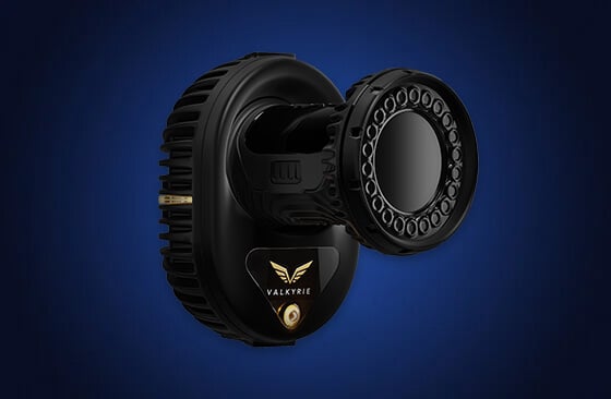
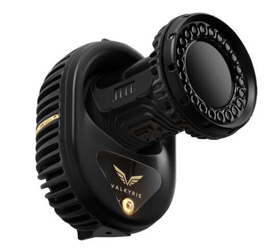
Valkyrie is the most powerful motion capture camera ever brought to market, offered with four different specs with four different focuses: resolution, speed, value, and strobeless.
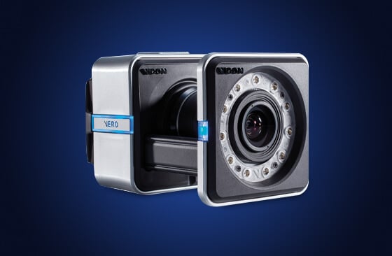
With the best resolution/speed/price offering on the market, Vicon Vero is the latest optical camera from Vicon. Building on the success of Vantage, Vero combined market-leading resolution and speed at an unrivaled price point. Like its bigger brother, Vantage, Vero has on-board sensors that monitor camera position and temperature to ensure optimal performance at all times.
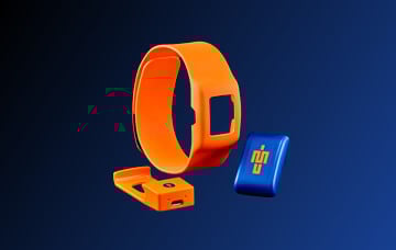
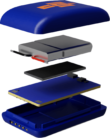
Engineered to capture the highest fidelity data, now you can fully integrate inertial into your optical world with Vicon – designed to work seamlessly together, Blue Trident allows you to capture the highest accelerations and global angles, and can be precisely synchronised with your optical data within Nexus.
With effortless plug and play technology, Beacon creates a synchronized wireless network with lightning-fast throughput and low latency. Use it to combine inertial measurement with Vicon’s world-class, optical motion capture system, through Nexus – and precisely synchronise your data sets.
Vicon are here to support you on your Motion Capture journey. We’re happy to provide more information, answer questions and help you find the solution you need. Get in touch with our experts today.